Next: Lid-driven cavity (FVM) Up: Simple example problems Previous: Hydraulic pipe system Contents
The lid-driven cavity is a well-known benchmark problem for viscous
incompressible fluid flow [96]. The geometry at stake is shown in Figure
![[*]](crossref.png) . We are dealing with a square cavity consisting of three rigid
walls with no-slip conditions and a lid moving with a tangential unit
velocity. The lower left corner has a reference static pressure of 0. We are
interested in the velocity and pressure distribution for a Reynolds number of
400.
. We are dealing with a square cavity consisting of three rigid
walls with no-slip conditions and a lid moving with a tangential unit
velocity. The lower left corner has a reference static pressure of 0. We are
interested in the velocity and pressure distribution for a Reynolds number of
400.
**
**   Structure: lid-driven cavity.
**   Test objective: incompressible, viscous, laminar, 3D fluid flow
**
*NODE,NSET=Nall
1,0.00000,0.00000,0.
...
*ELEMENT,TYPE=F3D6,ELSET=Eall
1,1543,1626,1624,3918,4001,3999
...
*NSET,NSET=Nin
1774,
...
*NSET,NSET=Nwall
1,
...
*NSET,NSET=N1
1374,
...
*BOUNDARY
Nall,3,3,0.
Nwall,1,2,0.
Nin,2,2,0.
1,8,8,0.
2376,8,8,0.
*MATERIAL,NAME=WATER
*DENSITY
1.
*FLUID CONSTANTS
,.25E-2,293.
*SOLID SECTION,ELSET=Eall,MATERIAL=WATER
*INITIAL CONDITIONS,TYPE=FLUID VELOCITY
Nall,1,0.
Nall,2,0.
Nall,3,0.
*INITIAL CONDITIONS,TYPE=PRESSURE
Nall,0.
**
*STEP,INCF=20000
*CFD,STEADY STATE,FEM
*BOUNDARY
Nin,1,1,1.
*NODE FILE,FREQUENCYF=200
VF,PSF
*END STEP
The input deck is listed above (this deck is also available
in the test suite as file liquid1.inp). Although the problem is
essentially 2-dimensional it was modeled as a 3-dimensional problem with unit
thickness since 2-dimensional fluid capabilities are not available in
CalculiX. The mesh (2D projection) is shown in Figure . It
consists of 6-node wedge elements. There is one element layer across the
thickness. This is sufficient, since the results do not vary in thickness
direction. The input deck starts with the coordinates of the nodes and the
topology of the elements. The element type for fluid volumetric elements is the same
as for structural elements with the C replaced by F (fluid): F3D6. The nodes
making up the lid and those belonging to the no-slip walls are collected into
the nodal sets Nin and Nwall, respectively. The nodal set N1 is created for
printing purposes. It contains a subset of nodes close to the lid.
The homogeneous boundary conditions (i.e. those with zero value) are listed next underneath the *BOUNDARY keyword: The velocity in all nodes in z-direction is zero, the velocity at the walls is zero (no-slip condition) as well as the normal velocity at the lid. Furthermore, the reference point in the lower left corner of the cavity has a zero pressure (node 1 and its corresponding node across the thickness 2376). The material definition consists of the density, the heat capacity and the dynamic viscosity. The density is set to 1. The heat capacity and dynamic viscosity are entered underneath the *FLUID CONSTANTS keyword. The heat capacity is not needed since the calculation is steady state, so its value here is irrelevant. The value of the dynamic viscosity was chosen such that the Reynolds number is 400. The Reynolds number is defined as velocity times length divided by the kinematic viscosity. The velocity of the lid is 1, its length is 1 and since the density is 1 the kinematic and dynamic viscosity coincide. Consequently, the kinematic viscosity takes the value 1/400. The material is assigned to the elements by means of the *SOLID SECTION card.
The unknowns of the problem are the velocity and static pressure. No thermal boundary conditions are provided, so the temperature is irrelevant. All initial values for the unknowns are set to 0 by means o the *INITIAL CONDITIONS,TYPE=FLUID VELOCITY and *INITIAL CONDITIONS,TYPE=PRESSURE cards. Notice that for the velocity the initial conditions have to be specified for each degree of freedom separately.
The step is as usual started with the *STEP keyword. The maximum number of increments, however, is for fluid calculations governed by the parameter INCF. For steady state FEM fluid calculations the keyword *CFD,STEADY STATE,FEM is to be used. The values underneath this line are not relevant for fluid calculations, since the increment size is automatically chosen such that the procedure is stable. The nonzero tangential velocity of the lid is entered underneath the *BOUNDARY card. Recall that non-homogeneous (i.e. nonzero) boundary conditions have to be defined within a step. The step ends with a nodal print request for the velocity VF and the static pressure PS. The printing frequency is defined to be 200 by means of the FREQUENCYF parameter. This means, that results will be stored every 200 increments.
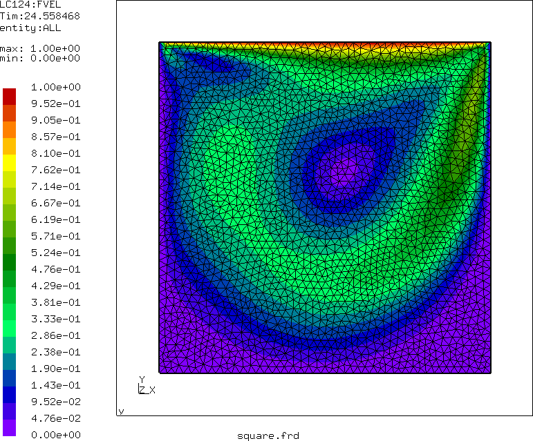
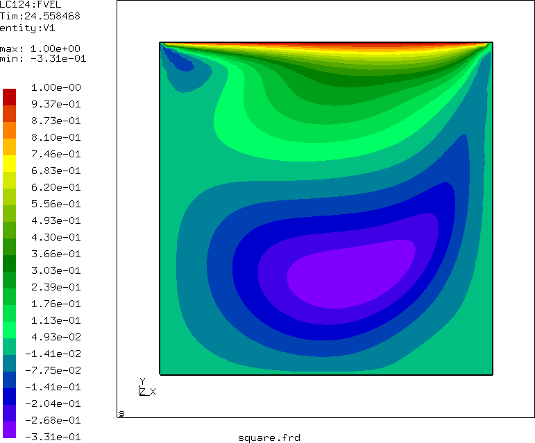
The velocity distribution in x-direction (i.e. the direction tangential to the lid) is
shown in Figure . The smallest value (-0.33) and its location
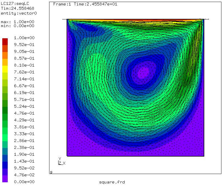
agree very well with the results in [96]. Figure
shows a vector plot of the velocity. Near the lid there is a large gradient,
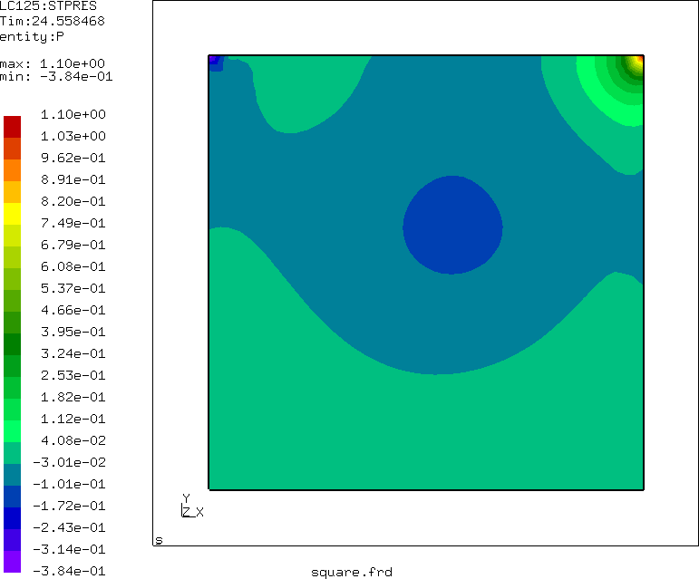
in the lower left and lower right corner are dead zones. The pressure plot
(Figure ) reveals a low pressure zone in the center of the major
vortex and in the left upper corner. The right upper corner is a stagnation
point for the x-component of the velocity and is characterized by a
significant pressure built-up.